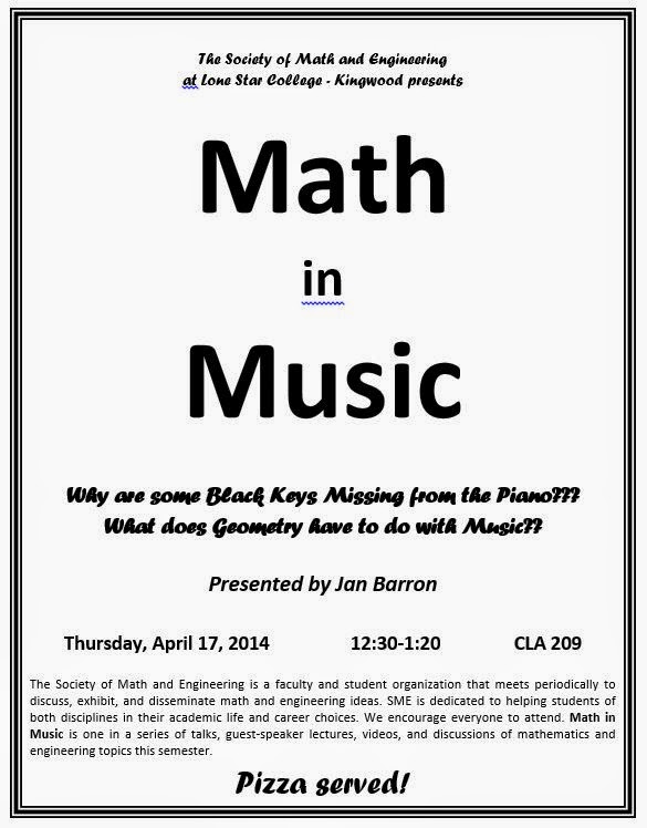
Don't forget - SME today!
https://blogger.googleusercontent.com/img/b/R29vZ2xl/AVvXsEhUnPJyja3tLlOYYq9-2NZnSSqIy4QQEVs7x7vDEmHJ27re_XrdsfcJ65CuO_uelbYvXPh_rwuph7Sejy0vmerTZmjeSqY3SWh3h2DVbPZ-iRzV6zwPna2mKf_ZatvsvO59dXHtG3l_Qas/s1600/SME.JPG
- Correct Formatting for Tables, Graphs & Calculations in Excel
Cheetah Example problem
If you can get everything set up for the Cheetah problem, you can copy and paste this format for the mousetrap car data.
I think most of you are becoming familiar with excel, but just in case... sorry, I should have gone through this at the beginning of the semester....
Housekeeping:
Double click on a sheet name, and rename it to better organize your working area:
Here, I have renamed "Sheet 2" to "Cheetah", and "Sheet 3" to "Mousetrap Car"
Use the (+) to add more sheets.
Get in the habit of using multiple sheets for a project to better organize your work.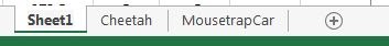
Double click on a sheet name, and rename it to better organize your working area:
Here, I have renamed "Sheet 2" to "Cheetah", and "Sheet 3" to "Mousetrap Car"
Use the (+) to add more sheets.
Get in the habit of using multiple sheets for a project to better organize your work.
#1 Set up your table
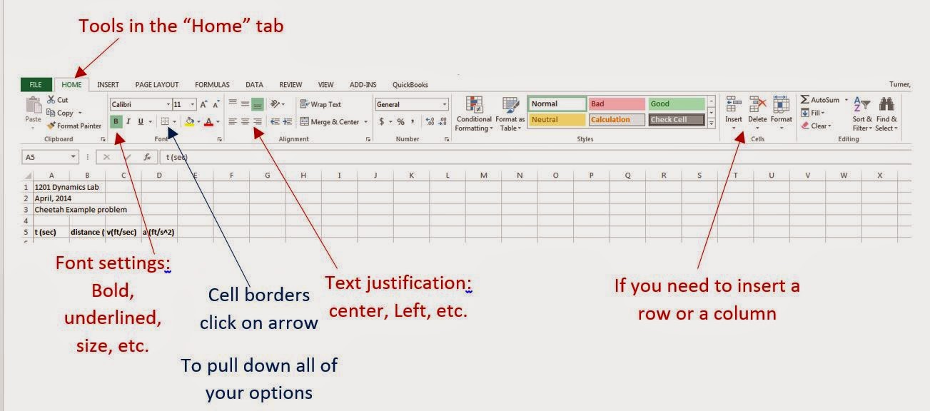
Use big bold font for headings
Add borders to cells, thick borders around Titles.
Center your text in the cells.
Set your precision (the number of decimals displayed) etc.
Note:
Just hover your mouse over the icons in the menu ribbon, wait for a second, and a little text box will appear with a description of the tool you are hovering over.
Some icons have a little arrow next to them, click on the arrow to see all of the different options available.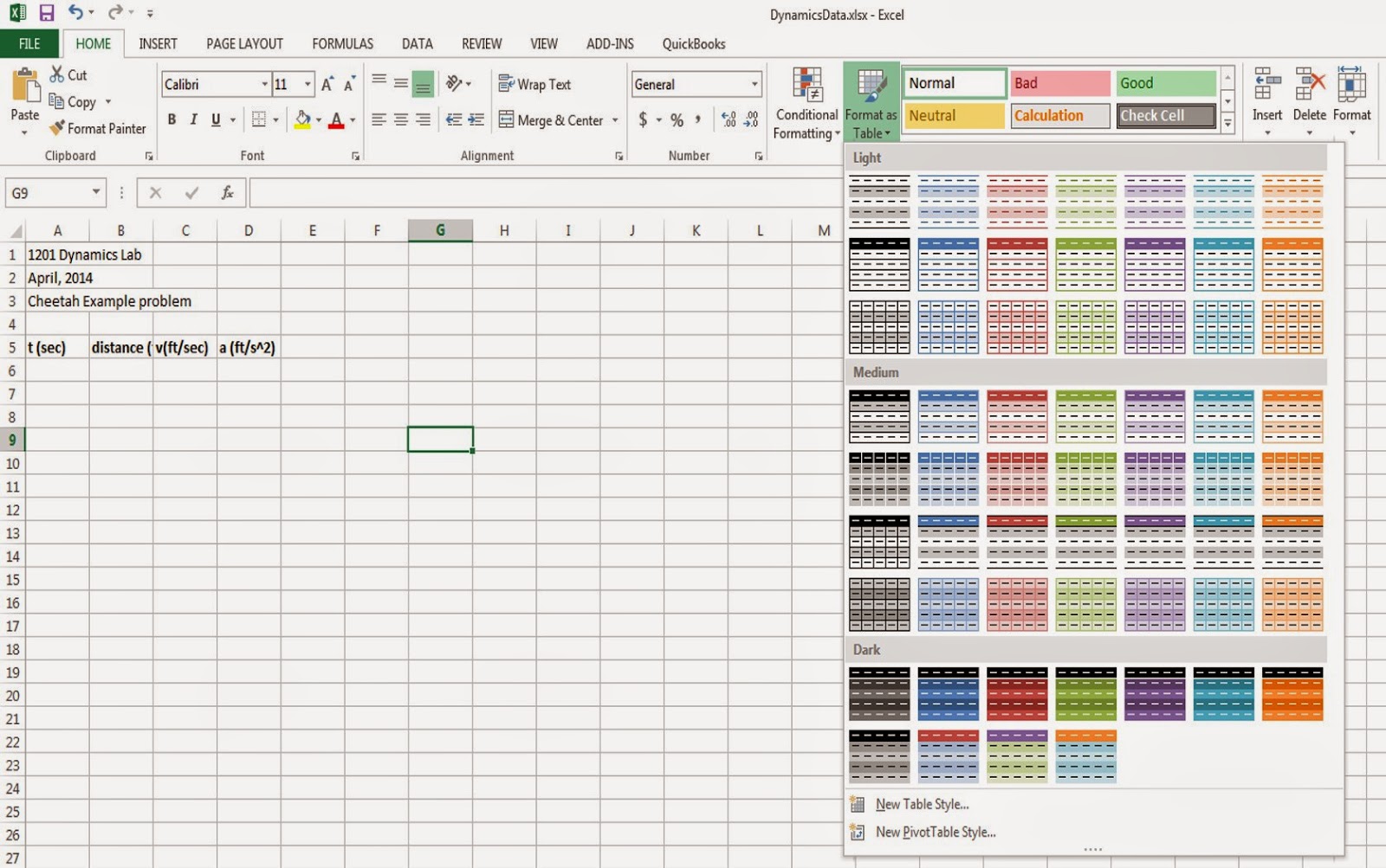
Test out some of the pre-made tables, but generally, you will want to make your own table (the colors look nice on the screen, but make it hard to print)
Don't forget to list the units you are using!

Printing:
I like to format everything for the printer right from the start (so I don't have to resize everything later).

Resize columns and rows so you can easily see data, and so your table is centered on your page:
Clicking on the upper left hand corner highlights all of your cells so you can format everything (like the font size, and precision) together: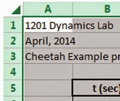
You can also select individual columns and rows to format: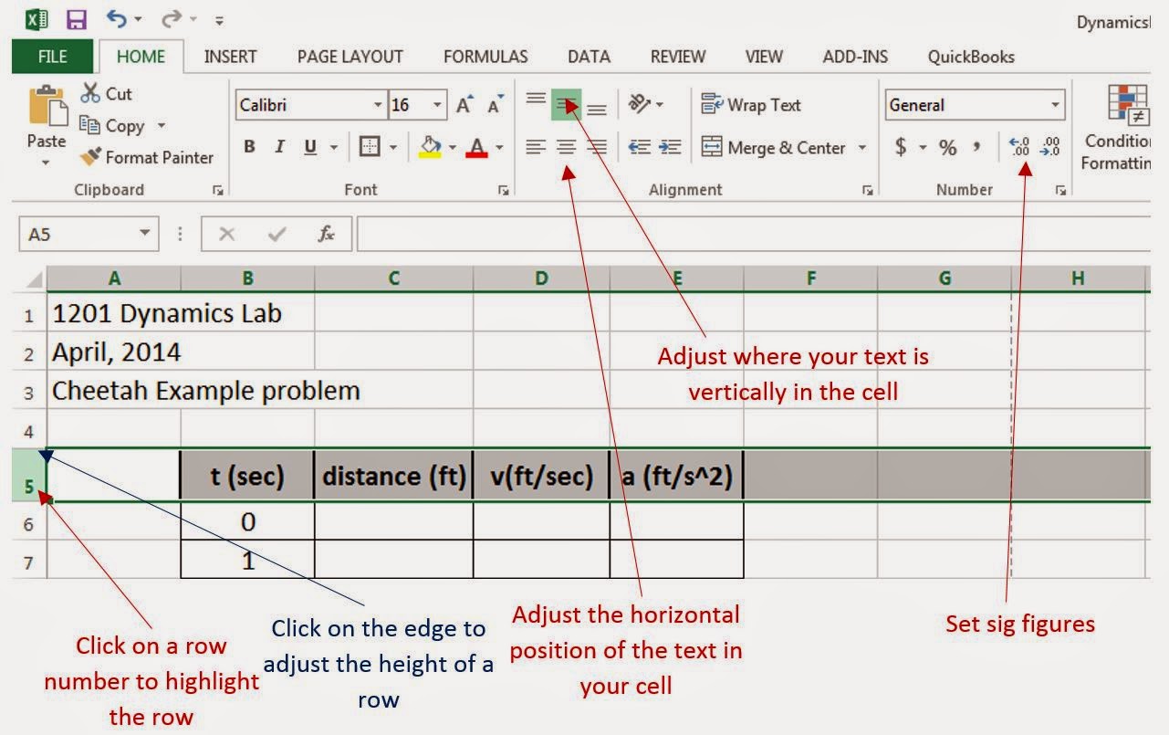
Same thing with columns, just click on a column (A, B, C) instead of a row.
I like to change the cell color in the top of the table to light grey: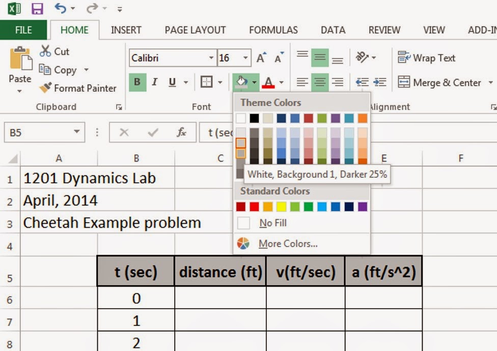
Not that everything is formatted correctly, it's time to start entering equations!
For the Cheetah problem:
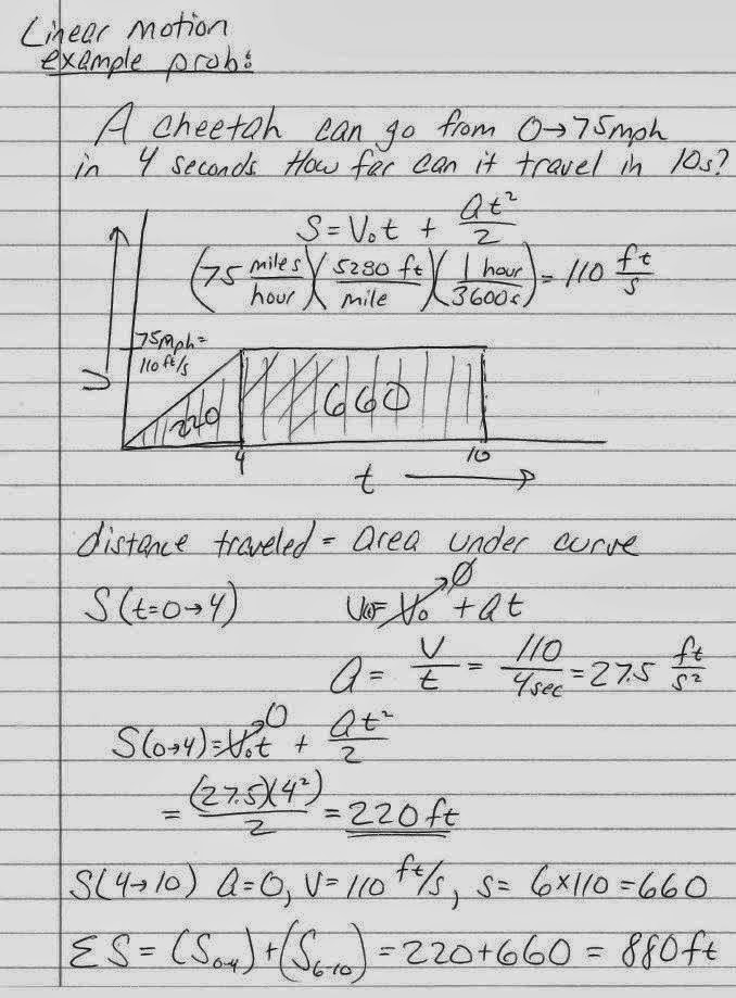
You don't need calculus to solve this, but know that this is one of the places calculus comes in handy if you have it!
Think about the graphs & how they relate to one another.
position vs. time → velocity = slope = ds/dt
Velocity vs. time →position = vel * time = (mph*h = m) = area under curve.
Velocity vs. time → acceleration = dV/dt = slope of V-t line
Acceleration vs. time → adt = dv (a = dv/dt)
Simplify areas under curves to being just triangles and rectangles...


Note: Often equations have constants in them that you want to define outside of the table.
Make a new table for initial position, velocity, and acceleration.
Rename the cells
c6→so
c7→vo
c8→ao
Just highlight the cell name, and type a new name into it. When you are referencing this value in your equation, you can now use a variable name, instead of a cell name.
Clicking on the upper left hand corner highlights all of your cells so you can format everything (like the font size, and precision) together:
You can also select individual columns and rows to format:
Same thing with columns, just click on a column (A, B, C) instead of a row.
I like to change the cell color in the top of the table to light grey:
Not that everything is formatted correctly, it's time to start entering equations!
For the Cheetah problem:
You don't need calculus to solve this, but know that this is one of the places calculus comes in handy if you have it!
Think about the graphs & how they relate to one another.
position vs. time → velocity = slope = ds/dt
Velocity vs. time →position = vel * time = (mph*h = m) = area under curve.
Velocity vs. time → acceleration = dV/dt = slope of V-t line
Acceleration vs. time → adt = dv (a = dv/dt)
Simplify areas under curves to being just triangles and rectangles...
Note: Often equations have constants in them that you want to define outside of the table.
Make a new table for initial position, velocity, and acceleration.
Rename the cells
c6→so
c7→vo
c8→ao
Just highlight the cell name, and type a new name into it. When you are referencing this value in your equation, you can now use a variable name, instead of a cell name.

Type in your equations:
Think of it just like typing something into your calculator.
Just highlight a cell, start with "=" and tell it what you want to do.
C11→0 Start with a distance of 0 (just type a zero in)
C12 → after your first time step, is where your first distance calculation will be. (how far has it gone in 1 second?)
Notice the color coding to keep track of what cells are in your equ.

Once you have an equation in one cell, you can copy it down to the other cells - just select the cell you have, grab the green square in the lower right hand corner, and drag it down.
Cells that you have renamed (like dt) will not change their value when you copy your equation down.
If you did not rename your cell, but you want it to be the same, use dollar signs.
$C$11 - will keep C11 through all calculations.
$C11 will keep "C" the same, but 11 will change to 12, 13, 14 etc. as you copy it.
Note the F4 key is the shortcut for adding dollar signs.
put your curser over the cell name in your equation
Hit F4 once for two dollar signs ($C$11)
Hit F4 again and again for other combinations ($C11, C$11, C11)
What the copied equations look like:
distance = (previous position) + 0.5 * acceleration * (time step)^2 + previous velocity * dt
Velocities = 2*(change in distance/change in time)-previous velocity
Look at the examples, calculate areas under curves, and make sure you understand how these equations relate to the graph!

The previous position changes for each calculation:
C11 = the previously calculated distance (so starting with 0, then going to the next time step etc.)
C12
C13
C14
Input equation for acceleration (a = dV/dt)
You should not have the first 4 seconds of your graph filled out: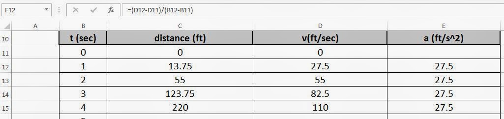
C13
C14
Input equation for acceleration (a = dV/dt)
You should not have the first 4 seconds of your graph filled out:
In the Cheetah problem (and for your mousetrap cars) there are different equations for different parts of your graph.
- has the acceleration changed? you might need a new equation!
Cheetah - after 4 sec, it stops accelerating, and instead maintains a constant speed of 110 ft/sec.
For the distance calculations starting at t = 5sec, acceleration is 0, and velocity is constant 110, so new distance = old distance + Vdt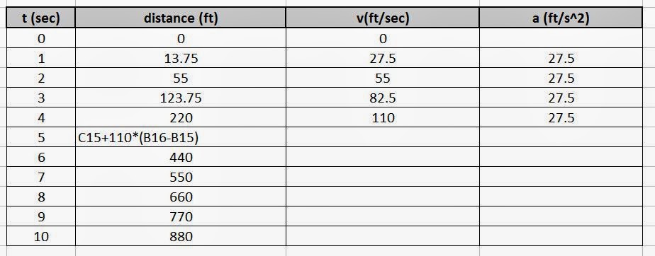
If your new distance is calculated correctly, can you just copy down the same v and a equations? try it out, think about it!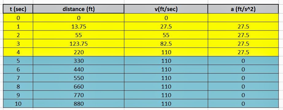
Don't forget to save your work when you have all the equations in correctly!
Now to graph out your data:
Highlight your entire table (including the titles t(sec), distance (ft), v(ft/sec), etc...
Insert →Chart→Scatter (xy) chart

Excel creates a default graph with 3 data sets (distance, velocity, and acceleration) all graphed against time.
Let's make three separate graphs, instead of one graph.
Copy the graph to make three graphs:
select graph, Ctrl+C, then Ctrl+V to paste.
Let's make three separate graphs, instead of one graph.
Copy the graph to make three graphs:
select graph, Ctrl+C, then Ctrl+V to paste.


Now we need to get rid of the legends, and add axis labels
x→time
y→distance, vel, acceleration etc.
Just select a graph, and click on the (+) to add axis titles.
Click on the paintbrush too to see editing tools there!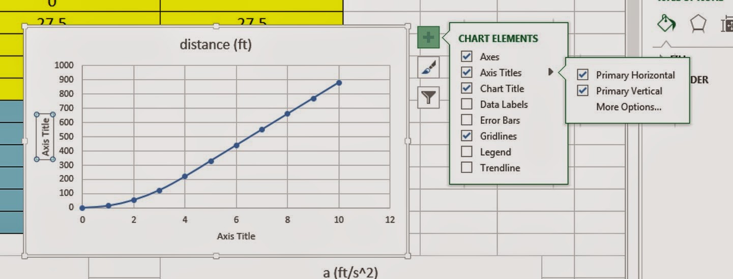
x→time
y→distance, vel, acceleration etc.
Just select a graph, and click on the (+) to add axis titles.
Click on the paintbrush too to see editing tools there!
Label all of your graphs correctly:

For your Mousetrap Car data, you will need to add a trend line to your graph.
Just select your line, right click on it, then select "add trendline"

If you select the trendline, there is a menu to let you display the equation, select what kind of a fit, etc.

When data is not perfect, it is better to calculate Vel and Acc off of a nice smooth trend line. Engineers use trendlines a lot!
Note,
R-squared = the coefficient of determination (a measure of how well the model fits the data). Perfect fit → R-squared = 1.
horrible fit → R-squared = 0
If you want, break your line up into two lines, one that is 0>t>4, and one for 4<t<10. Fit two different lines. times above 4 should fit perfectly to a linear line.
Note: Do you have a different version of Excel?
Just youtube it to figure it out!!
Youtube → search "How to create a graph in Excel 2009" etc.
Think of it like driving cars - once you can drive a toyota, you can drive a honda too, the basic ideas in all of the versions are the same, you just have to find where they moved all of the buttons to.
Error Propagation test:
Pretend that instead of calculating the distances in the cheetah problem, you measured them off a camera (like we are going to do with the mousetrap cars). Copy your Cheetah data, and change the displacements so that they are all a little wrong, and see what happens to your velocity and acceleration calculations.
What % does your velocity change by if your position is off by 5%? What % does your acceleration change by?
Artificially create both random (some higher, and some lower), and systematic errors (all distances larger, or smaller) errors, and see what this does to the rest of your calculations.
Copy your cheetah data into a new worksheet.
1. Insert a new column next to your old distance column
2. Copy your correct distances into the new column (just type in the numbers, do not use an equation to put them in)
3. Erase your old distance column (what V and a use to make calculations off of) and input an equation where the new column's distance is the old column + error.
- Make a table to generate random errors.
- to make a random number in excel type in = RAND()
Make a column of = RAND()
Another column = first column * multiplication factor (like 5)
Another column = insert 1 and -1's
Another column = 1st * 1 or -1 to add errors randomly to either side of original data.
You should notice that it doesn't take much error in your distance measurements to make your velocity and acceleration calculations go haywire! This is an example of "error propagation" issues, and you will run into it over and over again when taking data.
Create a fit to your distance with errors line, use this equation to make a new smoothed out distance column, and try your V and a calculations again.

No comments:
Post a Comment